Matlab Data
Visualization and Processing Software Package
A. Matlab with
graphic user interface for data processing and visualization
Note:
1.The Matlab data visualization and processing package is uder
continuous developement, therefore the actual matlab program
windows that you see at the beam line station may be a little different
from
those in this instruction.
2. All commands shown in bold, and
words/phases on the windows shown with underline.
At
12-ID-B, we use matlab-based software package to convert
the 2D X-ray scattering images to 1D curves, and also visualize
the 2D images and 1D
data sets. This matlab software package contains several graphic
user interface (GUI) programs for X-ray scattering data visualization
and analysis.
Here are the steps to set up the matlab software package at PCs at the
beamline, in case it crashes for whatever
reasons.
1.
Start Matlab on PC:
Double
-click the Matlab icon at the Desktop, you will get the Matlab Window
like Figure 1. From the Address bar, navigate to your data
folder. In the your Data Folder, you will have several folders, i.e.,
"SAXS" folder --for SAXS data; "WAXS"--for WAXS data; "PE"- for perkinAlmer detector
data; "Log"--log files for your image data measurements.
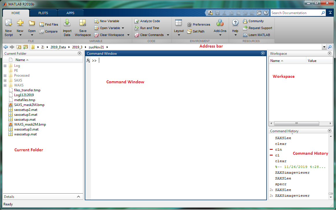
Figure 1.
Matlab program
window. "Current Folder" displays folders and files under your folder.
You can run matlab functions and commands in "Command Window" .
"Workspace" shows the matlab parameters in memory. "Command History"
displays commands/operations run recently in "Command Window"; you can
double-click the command to run it from the history list.
2.
Start 2-D Image Visualization Program Execute
(type and hit enter) “SAXSimageviewer”
in the matlab "Command
Window" and you will get the matlab graphic window "SAXSIMAGEVIEWER" for 2D
image visualization.
The command could also be run in the “Command History”
sub-window. Choose
an image data folder, for instance, "SAXS". Under menu "Plugin",
click "Experiment Setup", a matlab GUI program "GISAXSshop" will pop
up. More info on this GUI program see below. 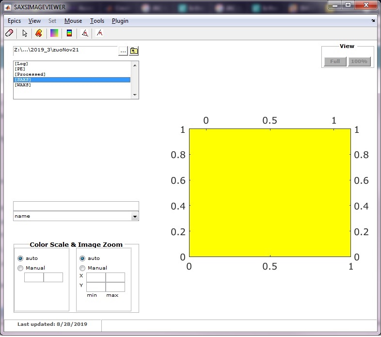
Figure 2.A
One can list images by "name", "date", "bytes", or "datenum". If listed by date, most recent ones stay at the top. 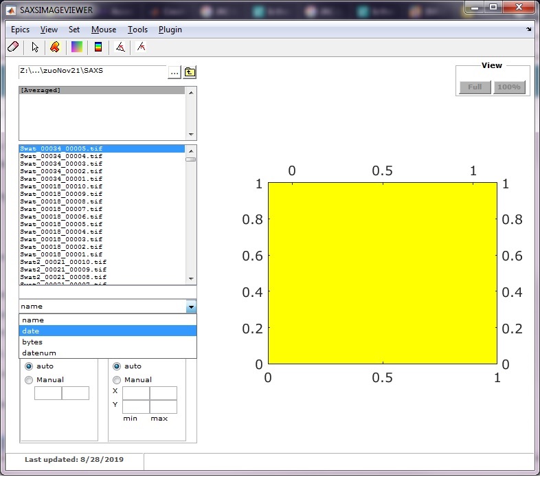
Figure 2.B Click any image file to display. Click
the square color icon to switch image color scales between log and
linear scales. This can also be done through "View" menu. There are choices of "auto" and "Manual" for Color Scale at left bottom. Manual option is recommended, with range of [0, 5]. There
are two choices, i.e., "auto" and "Manual", for Image Zoom.
"auto" will display the whole image; "Manual" will show specified area.
Holding left mouse on the image display, one can drag the image (pan
motion) while right mouse allow zooming in and out. Under
menu "Epics", you can specify image data from which detector
("Pilatus2M", "PerkinElmer", or "Mar 300") will be automatically
updated in the display window. 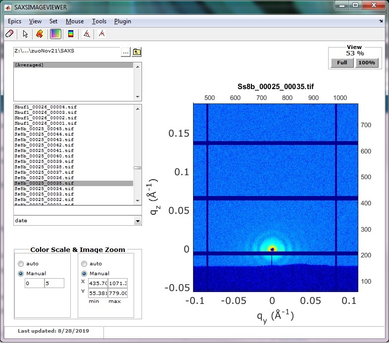
Figure 2.C Figure 2. The SAXSImageViewer program
screenshots (2.A,B,C). 3.
GISAXSshop ProgramThis
program is
needed for SAXSIMAGEVIEWER to correctly display 2D images. To start
it, click "Experiment Setup" from "Plugin" menu
in SAXSIMAGEVIEWER, or execute “gisaxsleenew” from "Command Window" or "Command History".
Either put parameters in "Experimental setup" or load them from botton
"Load setup info." if pre-saved info exists. After those experimental
setup information available,
the q_x, and q_y values will be computed and displayed in the 2D image
window (Figure 2.C). Then, the q value at every pixel will become
available and ready to check using mouse cursor. 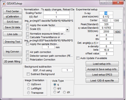
Figure 3. The GISAXSshop/"gisaxsleenew" program
screen.
4. 1D
Data Visualization
To
view the converted 1D profiles, type “SAXSLee”
and hit "Enter" key in the main matlab "Command Window"
and
you will get the following GUI program screen. Under the "File" menu,
click "Open Log File..."
to load the spec log file. The spec log file is starting with "Log",
followed by the first experimental date, for example, "Log11212019". Spec
log file contains records of sample measurements and motor scans. Do
NOT modify the spec log file! It may mess up data collection! When the
program loads the spec log file, it reads data file names from the spec
log
file. At 12-ID, 2-D images will be automatically converted to 1-D
curvers. Both will be saved to your data folder. Now, you
can
start to look
your 1-D data through "Select Data to Plot". The program screen also
provides other
functions, such as zooming, reading data point value, displaying
options
(linear, log), averaging and subtraction.
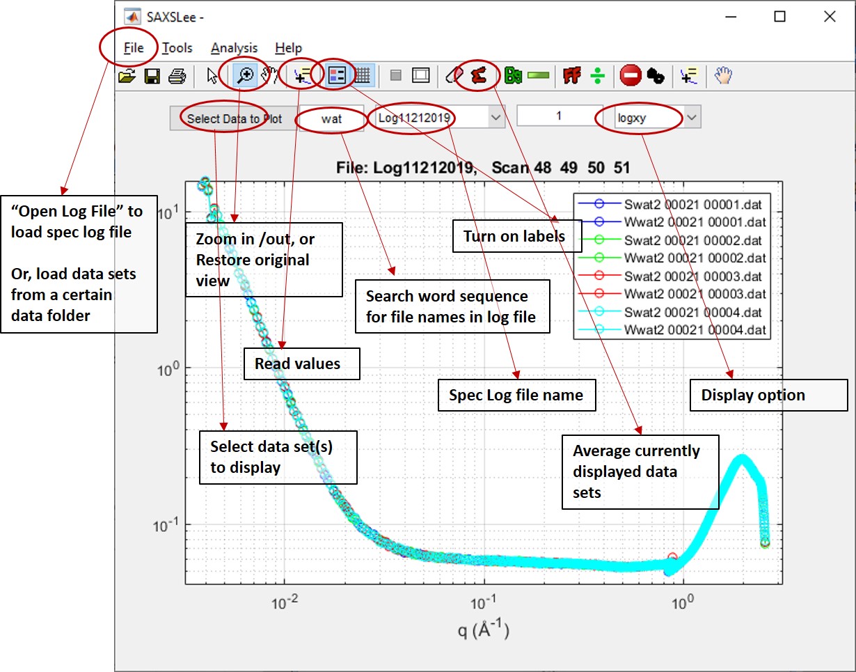
Figure 8. The SAXSLee program GUI.
5. View Motor
Scan Profile.
To view the
motor scan, type
"specr" in the main matlab "Command Window" and you will get the following
GUI program. Under the "File" menu, click "Open Log File" to load the spec log file, then you can start to look your data through "Select
Scan".
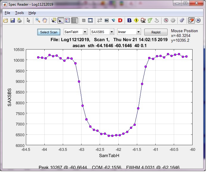
Figure 5. The specr GUI program.
B. Matlab
without graphics interface(!!Staff Use Only!!) --- for
automatic 2D image to 1D
profile conversion
At
12-ID-B, when the detectors collect images, they were
first saved on the detector computers, then transfered to network drive
and converted from 2D to 1D profiles. Image data can be
transferred and converted using computer "grape", or on the local linux
"purple". 1. 2D to 1D conversion using computer "grape" Log onto computer grape, start a linux terminal, run matlab >> matlab
-nosplash -nodisplay
this runs
the matlab without graphics >> SAXS_grape_server(detector_name) Choice of detector_name: 'pilatus2m', 'pilatus300k', 'pe' , 'mar300'
go back to spec terminal on computer Purple, load setup files, and start to collect image data. .. 2. 2D to 1D conversion using local computer "purple" On purple, open a new linux terminal,
[Purple]>>
cd
this leads to the home directory the
current computer user account
[Purple]>>
matlab
-nosplash -nodisplay
this runs
the matlab without graphics
Now,
we are in matlab workspace. go to you directory, for example, [in matlab]>>cd
/home/12id-b/2019_Data/2019_3/xxxx
load
the SAXS / WAXS setup files:
[in matlab]>>load
saxssetup.mat
[in matlab]>>load
waxssetup.mat
In matlab workspace, run "SAXSWAXSfiletransfer" and follow its instruction to enable automatic file
transfer and data
processing. Without setup files, it only transfer the files without
processing.
Note:
1. there may be two copies of matlab
running, one for data visualization (A. Matlab with graphic interface)
and one
for automatic data transfer and processing (B. Matlab without graphic
interface). Caution: "killall matlab" will terminate both
matlab programs.
C. Additional
instruction videos available:
|